CLOUD not ELSE : 2014

Wednesday, 31 December 2014

Aptitude Paper & solution - BE IT

All the students of BE IT kindly go through the following link.

1) Aptitude Paper-1
https://drive.google.com/file/d/0B4I4ScY2hV_7cDRtQVN1b0t0RFU/view?usp=sharing https://drive.google.com/file/d/0B4I4ScY2hV_7WWtzbjJrSXdYREU/view?usp=sharing

Solution for same paper-
https://drive.google.com/file/d/0B4I4ScY2hV_7WWtzbjJrSXdYREU/view?usp=sharing

Aptitude paper-2

Aptitude Paper- 2 with solution

Tuesday, 23 December 2014

ACN Study Material

Students will find here most of the pdf files of different subjects

https://drive.google.com/folderview?id=0B4I4ScY2hV_7T0VSN1BRcmQ1cWs&usp=sharing

Thursday, 11 December 2014

Algorithms- What does ‘Space Complexity’ mean?

Space Complexity:

Following are the correct definitions of Auxiliary Space and Space Complexity.

Auxiliary Space is the extra space or temporary space used by an algorithm.

Space Complexity of an algorithm is total space taken by the algorithm with respect to the input size. Space complexity includes both Auxiliary space and space used by input.

For example, if we want to compare standard sorting algorithms on the basis of space, then Auxiliary Space would be a better criteria than Space Complexity. Merge Sort uses O(n) auxiliary space, Insertion sort and Heap Sort use O(1) auxiliary space. Space complexity of all these sorting algorithms is O(n) though.

Algorithms- Solving Recurrences

Many algorithms are recursive in nature. When we analyze them, we get a recurrence relation for time complexity. We get running time on an input of size n as a function of n and the running time on inputs of smaller sizes. For example in Merge Sort, to sort a given array, we divide it in two halves and recursively repeat the process for the two halves. Finally we merge the results. Time complexity of Merge Sort can be written as T(n) = 2T(n/2) + cn. There are many other algorithms like Binary Search, Tower of Hanoi, etc.
There are mainly three ways for solving recurrences.
1) Substitution Method: We make a guess for the solution and then we use mathematical induction to prove the the guess is correct or incorrect.

For example consider the recurrence T(n) = 2T(n/2) + n

We guess the solution as T(n) = O(nLogn). Now we use induction
to prove our guess.

We need to prove that T(n) <= cnLogn. We can assume that it is true
for values smaller than n.

T(n) = 2T(n/2) + n
    <= cn/2Log(n/2) + n
    =  cnLogn - cnLog2 + n
    =  cnLogn - cn + n
    <= cnLogn

2) Recurrence Tree Method: In this method, we draw a recurrence tree and calculate the time taken by every level of tree. Finally, we sum the work done at all levels. To draw the recurrence tree, we start from the given recurrence and keep drawing till we find a pattern among levels. The pattern is typically a arithmetic or geometric series.

For example consider the recurrence relation 
T(n) = T(n/4) + T(n/2) + cn²

           cn²
         /      \
     T(n/4)     T(n/2)

If we further break down the expression T(n/4) and T(n/2), 
we get following recursion tree.

                cn²
           /           \      
       c(n²)/16      c(n²)/4
      /      \          /     \
  T(n/16)     T(n/8)  T(n/8)    T(n/4) 
Breaking down further gives us following
                 cn²
            /            \      
       c(n²)/16          c(n²)/4
       /      \            /      \
c(n²)/256   c(n²)/64  c(n²)/64    c(n²)/16
 /    \      /    \    /    \       /    \  

To know the value of T(n), we need to calculate sum of tree 
nodes level by level. If we sum the above tree level by level, 
we get the following series
T(n)  = c(n^2 + 5(n^2)/16 + 25(n^2)/256) + ....
The above series is geometrical progression with ratio 5/16.

To get an upper bound, we can sum the infinite series. 
We get the sum as (n²)/(1 - 5/16) which is O(n²)

3) Master Method:
Master Method is a direct way to get the solution. The master method works only for following type of recurrences or for recurrences that can be transformed to following type.

T(n) = aT(n/b) + f(n) where a >= 1 and b > 1

There are following three cases:
1. If f(n) = $\Theta \left(n^{{c}}\right)$ where c < $\log _{b}a$ then T(n) = $\Theta \left(n^{{\log _{b}a}}\right)$
2. If f(n) = $\Theta \left(n^{{c}}\right)$ where c = $\log _{b}a$ then T(n) = $\Theta \left(n^{{c}}logn\right)$
3.If f(n) = $\Theta \left(n^{{c}}\right)$ where c > $\log _{b}a$ then T(n) = $\Theta \left(f(n)\right)$
How does this work?
Master method is mainly derived from recurrence tree method. If we draw recurrence tree of T(n) = aT(n/b) + f(n), we can see that the work done at root is f(n) and work done at all leaves is $\Theta \left(n^{{c}}\right)$ where c is $\log _{b}a$ . And the height of recurrence tree is $\log _{b}n$

In recurrence tree method, we calculate total work done. If the work done at leaves is polynomially more, then leaves are the dominant part, and our result becomes the work done at leaves (Case 1). If work done at leaves and root is asymptotically same, then our result becomes height multiplied by work done at any level (Case 2). If work done at root is asymptotically more, then our result becomes work done at root (Case 3).
Examples of some standard algorithms whose time complexity can be evaluated using Master Method
Merge Sort: T(n) = 2T(n/2) + $\Theta(n)$ . It falls in case 2 as c is 1 and $\log _{b}a$ is also 1. So the solution is $\Theta(nLogn)$
Binary Search: T(n) = T(n/2) + $\Theta(1)$ . It also falls in case 2 as c is 0 and $\log _{b}a$ is also 0. So the solution is $\Theta(Logn)$
Notes:
1) It is not necessary that a recurrence of the form T(n) = aT(n/b) + f(n) can be solved using Master Theorem. The given three cases have some gaps between them. For example, the recurrence T(n) = 2T(n/2) + n/Logn cannot be solved using master method.
2) Case 2 can be extended for f(n) = $\Theta \left(n^{{c}}\log ^{{k}}n\right)$ .
If f(n) = $\Theta \left(n^{{c}}\log ^{{k}}n\right)$ for some constant k >= 0 and c = $\log _{b}a$ , then T(n) = $\Theta \left(n^{{c}}\log ^{{k+1}}n\right)$

Algorithms- Analysis of Loops

We have discussed Asymptotic Analysis, Worst, Average and Best Cases and Asymptotic Notations in previous posts. In this post, analysis of iterative programs with simple examples is discussed.
1) O(1): Time complexity of a function (or set of statements) is considered as O(1) if it doesn’t contain loop, recursion and call to any other non-constant time function.

   // set of non-recursive and non-loop statements

For example swap() function has O(1) time complexity.
A loop or recursion that runs a constant number of times is also considered as O(1). For example the following loop is O(1).

   // Here c is a constant   
   for (int i = 1; i <= c; i++) {  
        // some O(1) expressions
   }

2) O(n): Time Complexity of a loop is considered as O(n) if the loop variables is incremented / decremented by a constant amount. For example following functions have O(n) time complexity.

   // Here c is a positive integer constant   
   for (int i = 1; i <= n; i += c) {  
        // some O(1) expressions
   }

   for (int i = n; i > 0; i -= c) {
        // some O(1) expressions
   }

3) O(n^c): Time complexity of nested loops is equal to the number of times the innermost statement is executed. For example the following sample loops have O(n²) time complexity

  
   for (int i = 1; i <=n; i += c) {
       for (int j = 1; j <=n; j += c) {
          // some O(1) expressions
       }
   }

   for (int i = n; i > 0; i += c) {
       for (int j = i+1; j <=n; j += c) {
          // some O(1) expressions
   }

For example Selection sort and Insertion Sort have O(n²) time complexity.

4) O(Logn) Time Complexity of a loop is considered as O(Logn) if the loop variables is divided / multiplied by a constant amount.

   for (int i = 1; i <=n; i *= c) {
       // some O(1) expressions
   }
   for (int i = n; i > 0; i /= c) {
       // some O(1) expressions
   }

For example Binary Search(refer iterative implementation) has O(Logn) time complexity.

5) O(LogLogn) Time Complexity of a loop is considered as O(LogLogn) if the loop variables is reduced / increased exponentially by a constant amount.

   // Here c is a constant greater than 1   
   for (int i = 2; i <=n; i = pow(i, c)) { 
       // some O(1) expressions
   }
   //Here fun is sqrt or cuberoot or any other constant root
   for (int i = n; i > 0; i = fun(i)) { 
       // some O(1) expressions
   }

See this for more explanation.

How to combine time complexities of consecutive loops?
When there are consecutive loops, we calculate time complexity as sum of time complexities of individual loops.

   for (int i = 1; i <=m; i += c) {  
        // some O(1) expressions
   }
   for (int i = 1; i <=n; i += c) {
        // some O(1) expressions
   }
   Time complexity of above code is O(m) + O(n) which is O(m+n)
   If m == n, the time complexity becomes O(2n) which is O(n).

How to calculate time complexity when there are many if, else statements inside loops?
As discussed here, worst case time complexity is the most useful among best, average and worst. Therefore we need to consider worst case. We evaluate the situation when values in if-else conditions cause maximum number of statements to be executed.
For example consider the linear search function where we consider the case when element is present at the end or not present at all.
When the code is too complex to consider all if-else cases, we can get an upper bound by ignoring if else and other complex control statements.

How to calculate time complexity of recursive functions?
Time complexity of a recursive function can be written as a mathematical recurrence relation. To calculate time complexity, we must know how to solve recurrences. We will soon be discussing recurrence solving techniques as a separate post.

Algorithm - Asymptotic Notations

We have discussed Asymptotic Analysis, and Worst, Average and Best Cases of Algorithms. The main idea of asymptotic analysis is to have a measure of efficiency of algorithms that doesn’t depend on machine specific constants, and doesn’t require algorithms to be implemented and time taken by programs to be compared. Asymptotic notations are mathematical tools to represent time complexity of algorithms for asymptotic analysis. The following 3 asymptotic notations are mostly used to represent time complexity of algorithms.

1) $\Theta$ Notation: The theta notation bounds a functions from above and below, so it defines exact asymptotic behavior.
A simple way to get Theta notation of an expression is to drop low order terms and ignore leading constants. For example, consider the following expression.
3n³ + 6n² + 6000 = $\Theta$ (n³)
Dropping lower order terms is always fine because there will always be a n0 after which $\Theta$ (n³) beats $\Theta$ (n²) irrespective of the constants involved.
For a given function g(n), we denote $\Theta$ (g(n)) is following set of functions.

((g(n)) = {f(n): there exist positive constants c1, c2 and n0 such that
                  0 <= c1*g(n) <= f(n) <= c2*g(n) for all n >= n0}

The above definition means, if f(n) is theta of g(n), then the value f(n) is always between c1*g(n) and c2*g(n) for large values of n (n >= n0). The definition of theta also requires that f(n) must be non-negative for values of n greater than n0.

2) Big O Notation: The Big O notation defines an upper bound of an algorithm, it bounds a function only from above. For example, consider the case of Insertion Sort. It takes linear time in best case and quadratic time in worst case. We can safely say that the time complexity of Insertion sort is O(n^2). Note that O(n^2) also covers linear time.
If we use $\Theta$ notation to represent time complexity of Insertion sort, we have to use two statements for best and worst cases:
1. The worst case time complexity of Insertion Sort is $\Theta$ (n^2).
2. The best case time complexity of Insertion Sort is $\Theta$ (n).
The Big O notation is useful when we only have upper bound on time complexity of an algorithm. Many times we easily find an upper bound by simply looking at the algorithm.

O(g(n)) = { f(n): there exist positive constants c and n0 such that 
            0 <= f(n) <= cg(n) for all n >= n0}

3) $\Omega$ Notation: Just as Big O notation provides an asymptotic upper bound on a function, $\Omega$ notation provides an asymptotic lower bound.
$\Omega$ Notation< can be useful when we have lower bound on time complexity of an algorithm. As discussed in the previous post, the best case performance of an algorithm is generally not useful, the Omega notation is the least used notation among all three.
For a given function g(n), we denote by $\Omega$ (g(n)) the set of functions.

 (g(n)) = {f(n): there exist positive constants c and n0 such that 
                            0 <= cg(n) <= f(n) for all n >= n0}.

Let us consider the same Insertion sort example here. The time complexity of Insertion Sort can be written as $\Omega$ (n), but it is not a very useful information about insertion sort, as we are generally interested in worst case and sometimes in average case.

Algorithm- Worst, Average and Best Cases

In the previous post, we discussed how Asymptotic analysis overcomes the problems of traditional way of analyzing algorithms. In this post, we will take an example of Linear Search and analyze it using Asymptotic analysis.
We can have three cases to analyze an algorithm:
1) Worst Case
2) Average Case
3) Best Case
Let us consider the following implementation of Linear Search.

#include <stdio.h>

// Linearly search x in arr[].  If x is present then return the index,

// otherwise return -1

int search(int arr[], int n, int x)

{

    int i;

    for (i=0; i<n; i++)

    {

       if (arr[i] == x)

         return i;

    }

    return -1;

}

/* Driver program to test above functions*/

int main()

{

    int arr[] = {1, 10, 30, 15};

    int x = 30;

    int n = sizeof(arr)/sizeof(arr[0]);

    printf("%d is present at index %d", x, search(arr, n, x));

    getchar();

    return 0;

}

Worst Case Analysis (Usually Done)

In the worst case analysis, we calculate upper bound on running time of 
an algorithm. We must know the case that causes maximum number of 
operations to be executed. For Linear Search, the worst case happens 
when the element to be searched (x in the above code) is not present in 
the array.  When x is not present, the search() functions compares it 
with all the elements of arr[] one by one. Therefore, the worst case 
time complexity of linear search would be .

Average Case Analysis (Sometimes done) 

In average case analysis, we take all possible inputs and calculate 
computing time for all of the inputs.  Sum all the calculated values and
 divide the sum by total number of inputs. We must know (or predict) 
distribution of cases. For the linear search problem, let us assume that
 all cases are uniformly distributed
 (including the case of x not being present in array). So we sum all the
 cases and divide the sum by (n+1).  Following is the value of average 
case time complexity.

Average Case Time = 

                  =   

                  =    
 
Best Case Analysis (Bogus) 

In the best case analysis, we calculate lower bound on running time of 
an algorithm. We must know the case that causes minimum number of 
operations to be executed. In the linear search problem, the best case 
occurs when x is present at the first location. The number of operations
 in the best case is constant (not dependent on n). So time complexity 
in the best case would be 

Most of the times, we do worst case analysis to analyze algorithms.  In 
the worst analysis, we guarantee an upper bound on the running time of 
an algorithm which is good information.

The average case analysis is not easy to do in most of the practical 
cases and it is rarely done.  In the average case analysis, we must know
 (or predict) the mathematical distribution of all possible inputs.

The Best Case analysis is bogus.  Guaranteeing a lower bound on an 
algorithm doesn’t provide any information as in the worst case, an 
algorithm may take years to run.

For some algorithms, all the cases are asymptotically same, i.e., there are no worst and best cases.  For example, Merge Sort.  Merge Sort does operations
 in all cases. Most of the other sorting algorithms have worst and best 
cases.  For example, in the typical implementation of Quick Sort (where 
pivot is chosen as a corner element), the worst occurs when the input 
array is already sorted and the best occur when the pivot elements 
always divide array in two halves.  For insertion sort, the worst case 
occurs when the array is reverse sorted and the best case occurs when 
the array is sorted in the same order as output.

Algorithms

Why performance analysis?
There are many important things that should be taken care of, like user friendliness, modularity, security, maintainability, etc. when we check the performance .

Given two algorithms for a task, how do we find out which one is better?
One naive way of doing this is – implement both the algorithms and run the two programs on your computer for different inputs and see which one takes less time. There are many problems with this approach for analysis of algorithms.
1) It might be possible that for some inputs, first algorithm performs better than the second. And for some inputs second performs better.
2) It might also be possible that for some inputs, first algorithm perform better on one machine and the second works better on other machine for some other inputs.
Asymptotic Analysis is the big idea that handles above issues in analyzing algorithms. In Asymptotic Analysis, we evaluate the performance of an algorithm in terms of input size (we don’t measure the actual running time). We calculate, how does the time (or space) taken by an algorithm increases with the input size.
For example, let us consider the search problem (searching a given item) in a sorted array. One way to search is Linear Search (order of growth is linear) and other way is Binary Search (order of growth is logarithmic). To understand how Asymptotic Analysis solves the above mentioned problems in analyzing algorithms, let us say we run the Linear Search on a fast computer and Binary Search on a slow computer. For small values of input array size n, the fast computer may take less time. But, after certain value of input array size, the Binary Search will definitely start taking less time compared to the Linear Search even though the Binary Search is being run on a slow machine. The reason is the order of growth of Binary Search with respect to input size logarithmic while the order of growth of Linear Search is linear. So the machine dependent constants can always be ignored after certain values of input size.
Does Asymptotic Analysis always work?
Asymptotic Analysis is not perfect, but that’s the best way available for analyzing algorithms. For example, say there are two sorting algorithms that take 1000nLogn and 2nLogn time respectively on a machine. Both of these algorithms are asymptotically same (order of growth is nLogn). So, With Asymptotic Analysis, we can’t judge which one is better as we ignore constants in Asymptotic Analysis.
Also, in Asymptotic analysis, we always talk about input sizes larger than a constant value. It might be possible that those large inputs are never given to your software and an algorithm which is asymptotically slower, always performs better for your particular situation. So, you may end up choosing an algorithm that is Asymptotically slower but faster for your software.

Wednesday, 10 December 2014

The Software-Defined Data Center

Software-Defined Data Center.

May also be called software-defined datacenter (SDD) or virtual data center. Software-defined data center (SDDC) is the phrase used to refer to a data center where all infrastructure is virtualized and delivered as a service.
Control of the data center is fully automated by software, meaning hardware configuration is maintained through intelligent software systems. This is in contrast to traditional data centers where the infrastructure is typically defined by hardware and devices.
Software-defined data centers are considered by many to be the next step in the evolution of virtualization and cloud computing as it provides a solution to support both legacy enterprise applications and new cloud computing services.

We need to first see what sort of the changes has been made in SDDC-
On Following important aspects

Compute Virtualization

Modern software-defined compute (also known as server virtualization or simply “virtualization”) is the first step toward the Software-Defined Data Center. Introduced by VMware more than a decade ago, virtualization has become a standard technology implemented by the vast majority of data centers worldwide.
Conventionally deployed servers operate at less than 15 percent of capacity. Virtualization rewrites the entire equation. CPU and memory are decoupled from physical hardware, creating pools of resources for use wherever needed. Each virtualized application and its operating system are encapsulated in a separate, fully isolated software container called a virtual machine (VM). Many VMs can be run simultaneously on each server, putting the majority of hardware capacity to productive use. The results are transformative:

Superior performance
Higher availability
Significant savings

In the simplest terms, IT achieves a lot more with a lot less, at dramatically lower cost.

- See more at: http://www.vmware.com/software-defined-datacenter/compute.html#sthash.3mS6WjsR.dpuf

1) Computer Virtualization -
Modern software-defined compute (also known as server virtualization or simply “virtualization”) is the first step toward the Software-Defined Data Center. Introduced by VMware more than a decade ago, virtualization has become a standard technology implemented by the vast majority of data centers worldwide.
Conventionally deployed servers operate at less than 15 percent of capacity. Virtualization rewrites the entire equation. CPU and memory are decoupled from physical hardware, creating pools of resources for use wherever needed. Each virtualized application and its operating system are encapsulated in a separate, fully isolated software container called a virtual machine (VM). Many VMs can be run simultaneously on each server, putting the majority of hardware capacity to productive use. The results are trans formative:

Superior performance
Higher availability
Significant savings

In the simplest terms, IT achieves a lot more with a lot less, at dramatically lower cost.
2) Network Virtualization vs. Software-Defined Networking (SDN) -

As with server virtualization before it, network virtualization is a transformative architecture from VMware that overcomes previous limitations to deliver unprecedented performance, flexibility and economics.
In contrast to software-defined networking (SDN), in which hardware remains the driving force, VMware technology truly decouples network resources from underlying hardware. Virtualization principles are applied to physical network infrastructure, abstracting network services to create a flexible pool of transport capacity that can be allocated, utilized and repurposed on demand.
In a close analogy to the virtual machine, a virtual network is a software container that presents logical network components—logical switches, routers, firewalls, load balancers, VPNs and more—to connected workloads. These virtual networks are programmatically created, provisioned and managed, with the underlying physical network serving as a simple packet-forwarding backplane. Network and security services are allocated to each VM according to its needs, and stay attached to it as the VM moves among hosts in the dynamic virtualized environment. - See more at: http://www.vmware.com/software-defined-datacenter/networking-security.html#sthash.WPpi6YAC.dpuf

As with server virtualization before it, network virtualization is a transformative architecture from VMware that overcomes previous limitations to deliver unprecedented performance, flexibility and economics.

In contrast to software-defined networking (SDN), in which hardware remains the driving force, VMware technology truly decouples network resources from underlying hardware. Virtualization principles are applied to physical network infrastructure, abstracting network services to create a flexible pool of transport capacity that can be allocated, utilized and repurposed on demand.

In a close analogy to the virtual machine, a virtual network is a software container that presents logical network components—logical switches, routers, firewalls, load balancers, VPNs and more—to connected workloads. These virtual networks are programmatically created, provisioned and managed, with the underlying physical network serving as a simple packet-forwarding backplane. Network and security services are allocated to each VM according to its needs, and stay attached to it as the VM moves among hosts in the dynamic virtualized environment.

3)Software-Defined Storage (SDS)

Software-Defined Storage (SDS) is the vision that storage services are dynamically created and delivered per VM and controlled by policy. VMware’s SDS model shifts the operational model of storage from the bottoms-up array-centric approach of today’s storage to a tops-down VM-centric model. As a result storage services are precisely aligned with application requirements. - See more at: http://www.vmware.com/software-defined-datacenter/storage.html#sthash.0KdExNUj.dpuf

4)Unified Data Center Management Software

The fully virtualized data center is automated and managed by intelligent, policy-based data center management software, vastly simplifying governance and operations. A single, unified management platform lets you centrally monitor and administer all applications across physical geographies, heterogeneous infrastructure and hybrid clouds. You can deploy and manage workloads in physical, virtual and cloud environments with a unified management experience. IT becomes agile, elastic and responsive to a degree never before possible. - See more at: http://www.vmware.com/software-defined-datacenter/management.html#sthash.2VpYJfam.dpuf

Compute Virtualization

Modern software-defined compute (also known as server virtualization or simply “virtualization”) is the first step toward the Software-Defined Data Center. Introduced by VMware more than a decade ago, virtualization has become a standard technology implemented by the vast majority of data centers worldwide.

Conventionally deployed servers operate at less than 15 percent of capacity. Virtualization rewrites the entire equation. CPU and memory are decoupled from physical hardware, creating pools of resources for use wherever needed. Each virtualized application and its operating system are encapsulated in a separate, fully isolated software container called a virtual machine (VM). Many VMs can be run simultaneously on each server, putting the majority of hardware capacity to productive use. The results are transformative:

Superior performance
Higher availability
Significant savings

In the simplest terms, IT achieves a lot more with a lot less, at dramatically lower cost.

- See more at: http://www.vmware.com/software-defined-datacenter/compute.html#sthash.3mS6WjsR.dpuf

Saturday, 16 August 2014

ESDL- Creating Virtual Switches in the Hypervisor - Part-2

Dear All,

Here we will see the creation of vSwitch in Hypervisor (VMware ESXI-5.5)

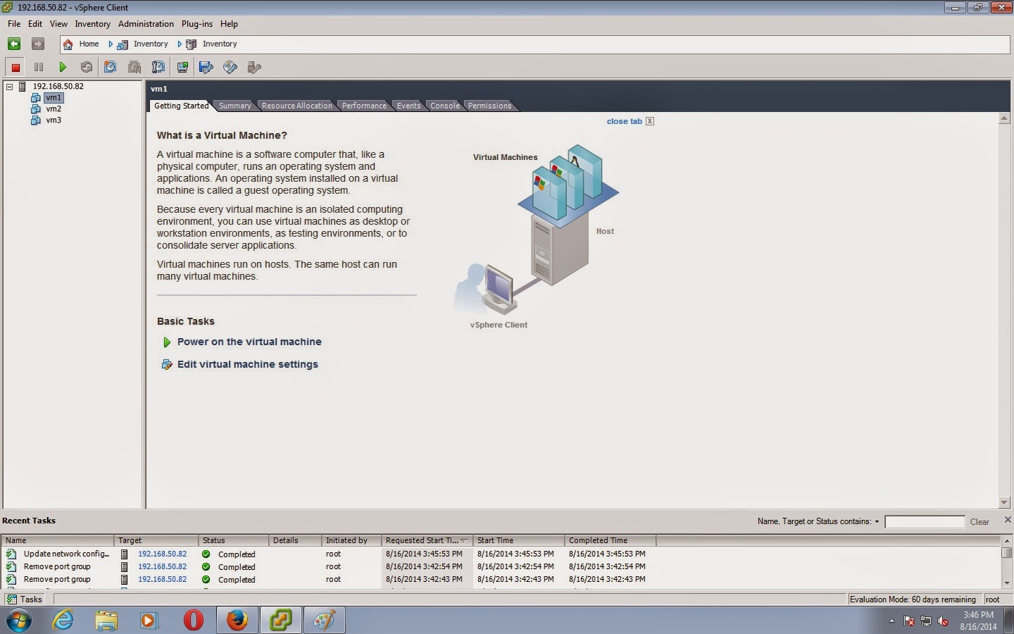
Step 1) It is same like to open the inventory from vsphere client with ESXI IP address username and password. Create atleast 3 VM.

Step2) Click on Inventory and click on Configuration in tab, you will get Hardware and software option
out of this select Networking that shows you the Management network has been connected with NIC card.

***** Here one thing plz keep in mind to install ESXi 5.5 on the server where two NIC cards has been installed so next steps that are related with creation of Virtual switches that is very easy.

Step3) Vswitch having a Management Netork only..

steps 4) Click on Add then one window come with below showing two options

step 5) Assign name and VLAN ID for respective virtual machine

step 6) Now that will automatically part of VSwitch 0.

Steps 7) Newly added vm is now a part of vswitch 0.

steps 8) go to the getting started tab.

step 9) select first VM and go to edit configuration settings. click on network adapter. Immediately Network labels will come select newly added network.

Steps 10) Same for VM2

Steps 10) Same for VM3

Steps 11) Now, they will be looking like below mentioned picture.

step 12) Now, we will create here New Virtual Switch

Step 13) Click on create vsphere standard switch - (Now vswitch 1 earlier vswitch 0)

Step 14) Assign Name and ID

Step 15) after assign the name and ID

steps 16) After creation of new VSwitch in hypervisor the following network connection will come.

At the last Second virtual Switch i.e. vSwitch1 does not content any physical address because the ESXi installed machine just have single NIC. If someone install ESXi on 2 NIC card available machine then vSwitch0 & vSwitch1 will connect with 2 different NIC.